spectrex mock example

End-to-end demonstration of the spectrex Phase 1 API using a synthetic (mock) scene on a 500 × 20 pixel NIRISS/GR150R grism stamp.

The pipeline:

1. Load instrument configuration and PCA eigenspectra basis

2. Build (or load) the sparse forward operator H

3. Generate a mock scene — sparse PCA coefficient vector ã

4. Forward-model: disperse ã through H to produce a grism image

5. Recover ã from the dispersed image by LSQR

6. Repeat with Poisson + read noise to demonstrate the realistic case

RMSE is computed on reconstructed flux values f(λ) = Φ @ a so it is physically meaningful and matches the parity plot axes.

from pathlib import Path

import matplotlib.pyplot as plt
import numpy as np

import spectrex
from spectrex import (
    EigenspectraBasis,
    InstrumentConfig,
    NoiseModel,
    SciPySparseOperator,
    SpectralSolver,
)

# ── Paths ────────────────────────────────────────────────────────────────────
TESTDATA = Path("../testdata")
OPERATOR_CACHE = Path("operator_cache.npz")

# ── Configuration ─────────────────────────────────────────────────────────────
COLD_START = False    # set True to force operator rebuild from scratch
IMAGE_SHAPE = (500, 20)
SOURCE_DENSITY = 0.1  # fraction of pixels with injected sources
SEED = 42
N_COMPONENTS = 10     # must match eigenspectra CSV

rng = np.random.default_rng(SEED)

print(f"spectrex {spectrex.__version__}")

spectrex 0.2.1.dev18+gc6f5edaa6.d20260506

Step 1 — Instrument configuration & eigenspectra basis

InstrumentConfig loads the aXe grism config file, wavelength range, and sensitivity curves. EigenspectraBasis loads the 10 Kurucz PCA eigenspectra and interpolates them onto the instrument wavelength grid.

config = InstrumentConfig.from_files(
    conf_path=TESTDATA / "Config Files" / "GR150R.F150W.220725.conf",
    wavelengthrange_path=TESTDATA / "jwst_niriss_wavelengthrange_0002.asdf",
    sensitivity_dir=TESTDATA / "SenseConfig" / "wfss-grism-configuration",
    filter_name="F150W",
    n_wavelengths=150,
)

basis = EigenspectraBasis.from_csv(
    TESTDATA / "eigenspectra_kurucz.csv",
    config.wavelengths,
)

print(f"Wavelength range: {config.wavelengths[0]:.0f} – {config.wavelengths[-1]:.0f} Å")
print(f"Grism orders: {list(config.orders)}")
print(f"Basis components: {basis.n_components}")

Wavelength range: 12900 – 17100 Å
Grism orders: ['A', 'B', 'C', 'D', 'E']
Basis components: 10

Step 2 — Forward operator

Builds the sparse matrix H (shape n_pix × n_pix·n_components) that maps PCA coefficients to dispersed pixel values across all grism orders.

Note: The first run builds H from scratch, which takes ~60 s for a 500 × 20 stamp. The result is cached to operator_cache.npz. Set COLD_START = True in the constants cell to force a rebuild.

import time

if OPERATOR_CACHE.exists() and not COLD_START:
    op = SciPySparseOperator.load(OPERATOR_CACHE)
    print(f"Operator loaded from {OPERATOR_CACHE}  "
          f"(shape {op._H.shape[0]} × {op._H.shape[1]})")
else:
    t0 = time.perf_counter()
    op = SciPySparseOperator.build(config, basis, IMAGE_SHAPE)
    op.save(OPERATOR_CACHE)
    elapsed = time.perf_counter() - t0
    print(f"Operator built in {elapsed:.1f} s — cached to {OPERATOR_CACHE}")
    print(f"Shape: {op._H.shape[0]} × {op._H.shape[1]}")

Operator loaded from operator_cache.npz  (shape 10000 × 100000)

Step 3 — Mock scene

We inject sources at a random 10 % of pixels. For each active pixel we draw random PCA coefficients, accept only if the reconstructed spectrum is non-negative (physical), and store them in the flat coefficient vector ã.

The direct image is the broadband integrated flux I(x,y) = ∫ a(x,y,λ) dλ, visualised as a 2-D stamp.

n_pix = IMAGE_SHAPE[0] * IMAGE_SHAPE[1]
n = basis.n_components

a_tilde = np.zeros(n_pix * n)

num_active = int(SOURCE_DENSITY * n_pix)
active_k = rng.choice(n_pix, size=num_active, replace=False)

MAX_TRIES = 50
n_placed = 0
for k in active_k:
    for _ in range(MAX_TRIES):
        flux = rng.uniform(-1, 1, size=n)
        if np.all(basis.reconstruct(flux) >= 0):
            a_tilde[k * n : (k + 1) * n] = flux
            n_placed += 1
            break

print(f"Sources placed: {n_placed} / {num_active} requested "
      f"({100 * n_placed / n_pix:.1f} % of pixels)")

direct = basis.broadband_image(a_tilde, IMAGE_SHAPE)
print(f"Direct image shape: {direct.shape},  max flux: {direct.max():.4f}")

Sources placed: 896 / 1000 requested (9.0 % of pixels)
Direct image shape: (500, 20),  max flux: 698067752.2096

Noiseless recovery

Forward-model ã → dispersed grism image, then recover ã from the dispersed image using LSQR. The support mask is built from the direct image (non-zero pixels) so LSQR only solves for active columns of H.

dispersed = op.apply(a_tilde).reshape(IMAGE_SHAPE)

# Support mask: True at pixels known to have a source
support_mask = a_tilde != 0
print(f"Dispersed image range: [{dispersed.min():.4f}, {dispersed.max():.4f}]")
print(f"Active coefficients:   {support_mask.sum()} / {len(support_mask)}")

Dispersed image range: [0.0000, 17101.3035]
Active coefficients:   8960 / 100000

solver = SpectralSolver(op, max_iter=500, tolerance=1e-8)
recovered = solver.solve(dispersed, support_mask=support_mask)
print(f"Recovered vector shape: {recovered.shape}")

Recovered vector shape: (100000,)

active_indices = [k for k in range(n_pix) if np.any(a_tilde[k * n : (k + 1) * n] != 0)]

true_flux = np.concatenate(
    [basis.reconstruct(a_tilde[k * n : (k + 1) * n]) for k in active_indices]
)
rec_flux = np.concatenate(
    [basis.reconstruct(recovered[k * n : (k + 1) * n]) for k in active_indices]
)

rmse_noiseless = np.sqrt(np.mean((true_flux - rec_flux) ** 2))
print(f"Noiseless RMSE (flux): {rmse_noiseless:.6f}")

Noiseless RMSE (flux): 21287.860870

def _clip(arr, nsigma_lo=2, nsigma_hi=2):
    m, s = np.nanmean(arr), np.nanstd(arr)
    return m - nsigma_lo * s, m + nsigma_hi * s

recovered_img = basis.broadband_image(recovered, IMAGE_SHAPE)
residual_img  = np.abs(direct - recovered_img)

vmin_dr, vmax_dr = _clip(direct)                       # shared scale for Direct & Recovered
vmin_d2, vmax_d2 = _clip(dispersed)
vmax_res = np.nanmean(residual_img) + np.nanstd(residual_img)

fig, axes = plt.subplots(1, 4, figsize=(14, 4))
kw = dict(origin="lower", aspect="auto", interpolation="nearest", cmap="inferno")

im0 = axes[0].imshow(direct,        vmin=vmin_dr, vmax=vmax_dr, **kw)
im1 = axes[1].imshow(dispersed,     vmin=vmin_d2, vmax=vmax_d2, **kw)
im2 = axes[2].imshow(recovered_img, vmin=vmin_dr, vmax=vmax_dr, **kw)
im3 = axes[3].imshow(residual_img,  vmin=0,       vmax=vmax_res, **kw)

titles = ["Direct image", "Dispersed (grism)", "Recovered", "|Residual|"]
for ax, im, title in zip(axes, [im0, im1, im2, im3], titles):
    ax.set_title(title)
    ax.set_xlabel("column")
    ax.set_ylabel("row")
    fig.colorbar(im, ax=ax, fraction=0.046, pad=0.04)

fig.suptitle("Noiseless recovery — 500 × 20 stamp, GR150R/F150W", y=1.01)
fig.tight_layout()
plt.show()

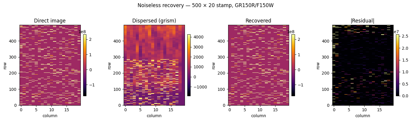
The dispersion process includes sources that do not reside entirely within the dispersed image due to positional shifts. This is an edge effect that we should include in a future version by virtually extending the pixel coordinates of the model image to negative and beyond the original size values in the dispersion direction.

fig, axes = plt.subplots(2, 1, figsize=(5, 8), sharex=True, tight_layout=True, height_ratios=(1, 0.6), gridspec_kw={'hspace': 0})
ax = axes[0]
outliers = rec_flux <= 1.

ax.scatter(true_flux[~outliers], rec_flux[~outliers], s=2, alpha=0.05, linewidths=0, color="C0", rasterized=True)
ax.scatter(true_flux[outliers], rec_flux[outliers], s=2, alpha=0.05, linewidths=0, color="C1", rasterized=True)
minv = max(min(true_flux.min(), rec_flux.min()), -10_000)
maxv = max(true_flux.max(), rec_flux.max())
ax.plot([minv, maxv], [minv, maxv], "r--", lw=1, label="1:1")
ax.set_aspect("equal", adjustable="box")
ax.set_xlim(minv, maxv)
ax.set_ylim(minv, maxv)
ax.set_ylabel("Recovered flux  f(λ)")
ax.set_title("Parity plot — noiseless")

ax = axes[1]
frac_residuals = (true_flux - rec_flux) / true_flux
ax.scatter(true_flux[~outliers], frac_residuals[~outliers], s=2, alpha=0.05, linewidths=0, color="C0", rasterized=True)
ax.scatter(true_flux[outliers], frac_residuals[outliers], s=2, alpha=0.05, linewidths=0, color="C1", rasterized=True)
ax.set_ylim(-2, 2)
ax.set_xlabel("True flux  f(λ)")
rmse_noiseless_good = np.sqrt(np.mean(frac_residuals[~outliers]) ** 2)
ax.text(0.05, 0.92, f"frac. mean error = {rmse_noiseless_good:.4f}", color='C0',
        transform=ax.transAxes, fontsize=10,
        bbox=dict(boxstyle="round,pad=0.3", fc="white", ec="gray", alpha=0.8))
fig.tight_layout()


plt.show()

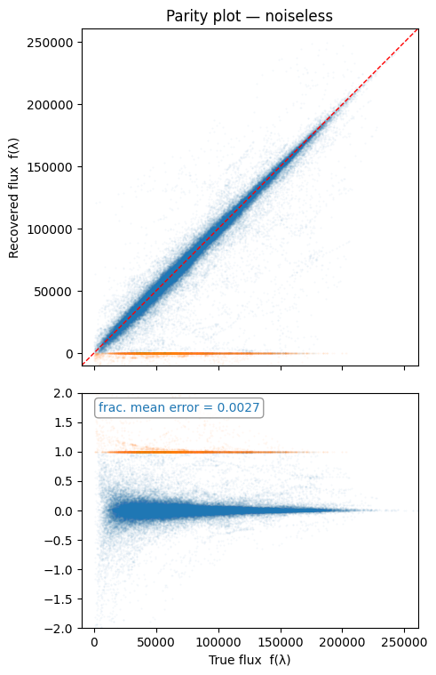
For this plot we highlight the failed recovery due to mapping coverage mentioned above. The fractional mean error is calculated without these outliers.

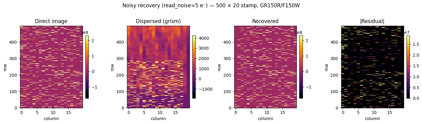
Noisy recovery

We add Gaussian noise approximating Poisson + detector read noise (read_noise = 5 e⁻) using NoiseModel.sample(). The same support mask and LSQR solver are used; the only change is the input image.

This is the realistic operating regime for real JWST data.

noise_model = NoiseModel(read_noise=5.0)
noisy_dispersed = noise_model.sample(dispersed, rng)
print(f"Noisy dispersed range: [{noisy_dispersed.min():.4f}, {noisy_dispersed.max():.4f}]")
print(f"Added noise std (mean over pixels): "
      f"{np.std(noisy_dispersed - dispersed):.4f}")

Noisy dispersed range: [-24.6412, 16906.7927]
Added noise std (mean over pixels): 34.1373

noisy_recovered = solver.solve(noisy_dispersed, support_mask=support_mask)
print(f"Noisy recovered vector shape: {noisy_recovered.shape}")

Noisy recovered vector shape: (100000,)

noisy_rec_flux = np.concatenate(
    [basis.reconstruct(noisy_recovered[k * n : (k + 1) * n]) for k in active_indices]
)

rmse_noisy = np.sqrt(np.mean((true_flux - noisy_rec_flux) ** 2))
print(f"Noiseless RMSE: {rmse_noiseless:.6f}")
print(f"Noisy RMSE:     {rmse_noisy:.6f}")
print(f"RMSE ratio:     {rmse_noisy / rmse_noiseless:.2f}×")

Noiseless RMSE: 21287.860870
Noisy RMSE:     25840.669446
RMSE ratio:     1.21×

noisy_recovered_img = basis.broadband_image(noisy_recovered, IMAGE_SHAPE)
noisy_residual_img  = np.abs(direct - noisy_recovered_img)

vmax_nres = np.nanmean(noisy_residual_img) + np.nanstd(noisy_residual_img)

fig, axes = plt.subplots(1, 4, figsize=(14, 4))

im0 = axes[0].imshow(direct,             vmin=vmin_dr,   vmax=vmax_dr,   **kw)
im1 = axes[1].imshow(noisy_dispersed,    vmin=vmin_d2,   vmax=vmax_d2,   **kw)
im2 = axes[2].imshow(noisy_recovered_img,vmin=vmin_dr,   vmax=vmax_dr,   **kw)
im3 = axes[3].imshow(noisy_residual_img, vmin=0,         vmax=vmax_nres, **kw)

for ax, im, title in zip(axes, [im0, im1, im2, im3], titles):
    ax.set_title(title)
    ax.set_xlabel("column")
    ax.set_ylabel("row")
    fig.colorbar(im, ax=ax, fraction=0.046, pad=0.04)

fig.suptitle("Noisy recovery (read_noise=5 e⁻) — 500 × 20 stamp, GR150R/F150W", y=1.01)
fig.tight_layout()
plt.show()

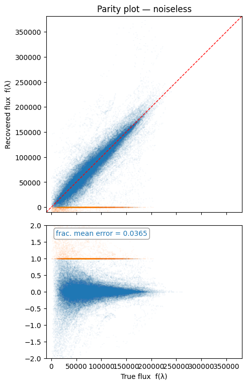
fig, axes = plt.subplots(2, 1, figsize=(5, 8), sharex=True, tight_layout=True, height_ratios=(1, 0.6), gridspec_kw={'hspace': 0})
ax = axes[0]
outliers = noisy_rec_flux <= 1.
minv = max(min(true_flux.min(), noisy_rec_flux.min()), -10_000)
maxv = max(true_flux.max(), noisy_rec_flux.max())
ax.scatter(true_flux[~outliers], noisy_rec_flux[~outliers], s=2, alpha=0.05, linewidths=0, color="C0", rasterized=True)
ax.scatter(true_flux[outliers], noisy_rec_flux[outliers], s=2, alpha=0.05, linewidths=0, color="C1", rasterized=True)
minv = max(min(true_flux.min(), noisy_rec_flux.min()), -10_000)
maxv = max(true_flux.max(), noisy_rec_flux.max())
ax.plot([minv, maxv], [minv, maxv], "r--", lw=1, label="1:1")
ax.set_aspect("equal", adjustable="box")
ax.set_xlim(minv, maxv)
ax.set_ylim(minv, maxv)
ax.set_ylabel("Recovered flux  f(λ)")
ax.set_title("Parity plot — noiseless")

ax = axes[1]
frac_residuals = (true_flux - noisy_rec_flux) / true_flux
ax.scatter(true_flux[~outliers], frac_residuals[~outliers], s=2, alpha=0.05, linewidths=0, color="C0", rasterized=True)
ax.scatter(true_flux[outliers], frac_residuals[outliers], s=2, alpha=0.05, linewidths=0, color="C1", rasterized=True)
ax.set_ylim(-2, 2)
ax.set_xlabel("True flux  f(λ)")
rmse_noiseless_good = np.sqrt(np.mean(frac_residuals[~outliers]) ** 2)
ax.text(0.05, 0.92, f"frac. mean error = {rmse_noiseless_good:.4f}", color='C0',
        transform=ax.transAxes, fontsize=10,
        bbox=dict(boxstyle="round,pad=0.3", fc="white", ec="gray", alpha=0.8))
fig.tight_layout()


plt.show()

Next steps

The parity plots above give a single RMSE figure for one source density. To quantify how recovery quality degrades as the field becomes more crowded, see the planned sweep notebook:

notebooks/analysis_rmse_vs_density.ipynb

That notebook will define a run_pipeline(a_tilde, op, basis, noise_model=None) helper and sweep SOURCE_DENSITY over ~5–8 values, plotting RMSE vs density for both the noiseless and noisy cases. This sweep is important for establishing the credibility of the method in crowded NIRISS fields.