Solvers

Spectral extraction reduces to recovering the source coefficient vector \(\mathbf{a}\) from the dispersed observation \(\mathbf{f}\) and the forward operator \(H\). spectrex provides two solver families with different trade-offs.

Noise Model

Weighted least squares requires pixel-level uncertainty estimates. NoiseModel models detector noise as

\[\sigma^2_p = \sigma_\text{read}^2 + \max(f_p, 0)\]

so that both read noise and Poisson photon noise contribute. The precision_weights() method returns \(1/\sigma_p\) for each pixel; these weights appear in the solver objectives as \(W = \mathrm{diag}(\boldsymbol{\sigma}^{-1})\).

SpectralSolver

SpectralSolver wraps scipy.sparse.linalg.lsqr() and scipy.sparse.linalg.lsmr() to solve the unconstrained weighted least-squares problem

\[\min_{\mathbf{a}} \| W (H\mathbf{a} - \mathbf{f}) \|_2^2\]

via solve(). solve_regularised() adds a Tikhonov term

\[\min_{\mathbf{a}} \| W (H\mathbf{a} - \mathbf{f}) \|_2^2 + \lambda \|\mathbf{a}\|_2^2\]

The method and rcond arguments are set at construction time via SpectralSolver. LSQR and LSMR converge to the same solution but LSMR often has better convergence behaviour on ill-conditioned problems.

Note

SpectralSolver does not impose non-negativity or group-sparsity constraints. For crowded fields where such regularisation matters, use JAXProximalSolver instead.

JAXProximalSolver

JAXProximalSolver runs FISTA (Beck & Teboulle 2009) with a group-L1 (group-Lasso) penalty, solving

\[\min_{\mathbf{a}} \frac{1}{2}\| W (H\mathbf{a} - \mathbf{f}) \|_2^2 + \lambda \sum_k \| \mathbf{a}_k \|_2\]

where \(\mathbf{a}_k\) is the coefficient vector for source group k. The group-L1 term promotes whole-source sparsity: sources absent from the scene are zeroed out rather than pushed to small coefficients.

The full FISTA loop is JIT-compiled via jax.lax.while_loop().

Adaptive restart (O’Donoghue & Candès 2015) resets the FISTA momentum coefficient whenever the gradient condition

\[\langle \mathbf{f}_k - \mathbf{y}_k,\; \mathbf{x}_k - \mathbf{x}_{k-1} \rangle > 0\]

is detected. This prevents momentum from accumulating in the wrong direction on ill-conditioned problems and typically improves convergence by one to two orders of magnitude in the first hundred iterations. Set restart=False at construction time to disable.

Early stopping — set tol > 0 to halt when the relative change in \(\|\mathbf{a}\|\) falls below tol between iterations.

Diagnostics — pass a callback callable to receive (iteration, a, residual) at each step; this is the mechanism used in the comparison notebooks to record the residual norm convergence curve.

Note

FISTA optimises a different objective than LSQR (group-L1 vs. \(\ell_2\)-only). The FISTA residual floor is therefore expected to be higher than LSQR’s; this is not a defect.

Regularisation

The regularisation term determines what structure is imposed on the recovered coefficients beyond fitting the data. \(\mathbf{a}\) is a stacked vector of K sub-vectors, one per source:

\[\mathbf{a} = [\mathbf{a}_1,\, \mathbf{a}_2,\, \ldots,\, \mathbf{a}_K] \qquad \mathbf{a}_k \in \mathbb{R}^M\]

where M is the number of PCA basis components (n_components). Three penalties are relevant for this problem:

Name	Penalty	Promotes
Ridge (Tikhonov)	\(\lambda \|\mathbf{a}\|_2^2 = \lambda \sum_k \sum_m a_{km}^2\)	No sparsity — smoothly shrinks all coefficients toward zero. Implemented in SpectralSolver.
Group lasso (current JAX)	\(\lambda \sum_k \|\mathbf{a}_k\|_2\)	Source sparsity — the entire coefficient vector \(\mathbf{a}_k\) is zeroed when the source is absent. Individual elements within a non-zero group are not independently zeroed. Implemented in JAXProximalSolver.
Lasso (planned)	\(\lambda \sum_k \|\mathbf{a}_k\|_1 = \lambda \sum_k \sum_m |a_{km}|\)	Coefficient sparsity — only a few basis components are active per source; the rest are driven to exactly zero. Planned for a future release.
Sparse group lasso (planned)	\(\alpha \sum_k \|\mathbf{a}_k\|_2 + (1-\alpha)\sum_k \|\mathbf{a}_k\|_1\)	Both: few active sources and few components per source. Planned for a future release.

Why is group lasso called “group-L1”?

The “L1” refers to the norm taken across groups, not within each group. Each source’s coefficient vector is first summarised by its Euclidean (L2) norm \(\|\mathbf{a}_k\|_2\) — a single non-negative scalar. Those K scalars are then summed linearly (L1 norm), not squared:

\[\lambda \sum_k \|\mathbf{a}_k\|_2 \;=\; \lambda \bigl\| \bigl(\|\mathbf{a}_1\|_2,\; \ldots,\; \|\mathbf{a}_K\|_2\bigr) \bigr\|_1\]

By contrast, the plain lasso uses the L1 norm directly on all elements, and ridge uses the squared L2 norm on all elements. The proximal operator for the group lasso (block soft-threshold) zeros out the entire \(\mathbf{a}_k\) when \(\|\mathbf{a}_k\|_2 \leq \lambda/L\); it never zeros a single element independently.

Which prior fits the spectral basis problem?

The original motivation for regularisation in spectrex is that a small number of PCA basis components should suffice to represent any stellar spectrum. That assumption is about sparsity within each source’s coefficient vector, which maps to the lasso penalty \(\sum_k \|\mathbf{a}_k\|_1\), not the group lasso.

The group lasso is the correct prior when many catalog positions are expected to be empty (source-level sparsity), i.e the relevant scenario for blind or weakly-constrained source detection.

The current JAXProximalSolver implements the group lasso, which is useful for source-level deblending in crowded fields but does not enforce sparsity in the spectral basis coefficients per source. Adding a lasso (and sparse-group-lasso) option is planned; see What’s Next.

Which Solver?

Benchmark Figures

RMSE comparison — LSQR vs FISTA on a 5-source crowded scene:

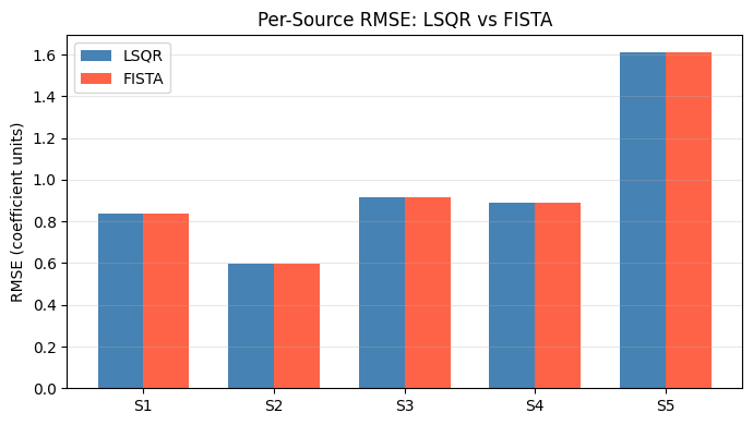
Fig. 1 Spectrum RMSE for LSQR vs FISTA on a 5-source crowded scene. Lower is better. See the Solver Accuracy Comparison: LSQR vs FISTA Group-L1 notebook for full methodology.

Weighted residual norm convergence over wall-clock time:

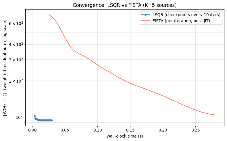
Fig. 2 Weighted residual norm \(\|W(Hx - f)\|\) vs wall-clock time. Short plateaus mark adaptive restart events (FISTA only). See the Computational Benchmarks: JAXOperator vs SciPySparseOperator notebook.

API Reference

class spectrex.NoiseModel(read_noise=5.0)

Bases: object

Poisson + read-noise model for JWST NIRISS detectors.

Parameters:

read_noise (float) – Detector read noise in electrons. Default 5.0.

precision_weights(f)

Precision weights 1 / σ(f) for whitening the linear system.

Parameters:

f (np.ndarray) – Observed pixel values.

Returns:

Positive weight array, same shape as f.

Return type:

np.ndarray

read_noise: float = 5.0

sample(f, rng)

Draw a noisy realisation of pixel values.

Adds zero-mean Gaussian noise with σ² = variance(f) to the input array. This is an approximation to Poisson + read noise suitable for mock data generation.

Parameters:

• f (np.ndarray) – Noiseless pixel values.

• rng (np.random.Generator) – NumPy random generator (e.g. np.random.default_rng(42)).

Returns:

Noisy pixel values with the same shape and dtype as f.

Return type:

np.ndarray

variance(f)

Per-pixel variance: σ²(f) = max(f, 0) + read_noise².

Parameters:

f (np.ndarray) – Observed pixel values (may be negative after sky subtraction).

Returns:

Non-negative variance, same shape as f.

Return type:

np.ndarray

class spectrex.SpectralSolver(operator, noise_model=None, regularisation=0.01, max_iter=1000, tolerance=1e-10)

Bases: object

Least-squares solver for WFSS spectral deconvolution.

Parameters:

• operator (ForwardOperatorProtocol) – The grism forward operator H. Any implementation satisfying the protocol is accepted (scipy or future JAX).

• noise_model (NoiseModel, optional) – Noise model for whitening in solve_regularised(). Uses uniform weights if None.

• regularisation (float) – Tikhonov regularisation parameter λ for solve_regularised(). Default 1e-2.

• max_iter (int) – Maximum solver iterations. Default 1000.

• tolerance (float) – Convergence tolerance (atol and btol). Default 1e-10.

solve(dispersed, support_mask=None)

LSQR solve for source coefficients.

Minimises ||H a - f||².

Parameters:

• dispersed (np.ndarray) – Dispersed detector image, shape image_shape.

• support_mask (np.ndarray, optional) – Boolean array, shape (n_coefficients,). When provided, the solve is restricted to True columns; the returned vector has zeros elsewhere.

Returns:

Coefficient vector a_tilde, shape (n_coefficients,).

Return type:

np.ndarray

solve_regularised(dispersed)

LSMR solve with Tikhonov regularisation and noise weighting.

Minimises ||W (H a - f)||² + λ ||a||² where W = diag(1/σ) from self.noise_model (identity if None).

Parameters:

dispersed (np.ndarray) – Dispersed detector image, shape image_shape.

Returns:

Coefficient vector a_tilde, shape (n_coefficients,).

Return type:

np.ndarray

class spectrex.JAXProximalSolver(operator, noise_model=None, lam=0.01, max_iter=200, lipschitz_n_iter=30, tol=0.0, restart=True, callback=None)

Bases: object

FISTA proximal gradient solver with group-L1 regularisation.

Minimises:

(1/2) ||W (H a - f)||² + λ Σ_k ||a_k||₂

where W = diag(precision_weights) and the group-L1 penalty zeros entire source groups (index k over basis components m).

The Lipschitz constant L of the gradient is estimated once at construction via power iteration; step size is 1/L. Convergence rate is O(1/k²) (Beck & Teboulle 2009).

Parameters:

• operator (ForwardOperatorProtocol) – The grism forward operator H.

• noise_model (NoiseModel, optional) – Noise model for precision weights. Uses uniform weights if None.

• lam (float) – Group-L1 regularisation strength λ. Default 1e-2.

• max_iter (int) – Maximum number of FISTA iterations. Default 200.

• lipschitz_n_iter (int) – Power iteration steps for step-size estimation. Default 30.

• tol (float) – Relative convergence tolerance. Stops early when ‖a_new − a‖ / (‖a‖ + 1e-10) < tol. Set to 0.0 (default) to always run max_iter iterations.

• restart (bool) – Enable gradient-based adaptive restart (O’Donoghue & Candès 2015). When the inner product ⟨∇f(y_k),  x_k − x_{k-1}⟩ is positive — indicating momentum overshoot — the momentum coefficient is reset to zero and iteration resumes from the current point. Default True.

• callback (callable, optional) – If provided, called at the end of every iteration as callback(iter, x, weighted_residual) where iter is 1-indexed, x is the current coefficient array (do not mutate), and weighted_residual is ‖W(Hx − f)‖. Adds one extra apply() call per iteration when set. Default None.

Notes

Why gradient restart, not monotone FISTA or backtracking? Gradient restart costs one dot product per iteration (O(K*M)). Monotone FISTA (MFISTA) requires an extra apply() call every time the objective increases; backtracking requires 1–3 extra calls per step. For NIRISS WFSS data, H^T W² H is ill-conditioned (bright and faint sources coexist; overlapping traces; precision weights spanning orders of magnitude). In this regime vanilla FISTA momentum overshoots the minimiser. Restart directly addresses this failure mode at negligible cost.

Why fixed step 1/L, not backtracking? power_iteration with 30 steps gives an accurate Lipschitz estimate for JAX operators. Backtracking is only warranted when the estimate is unreliable; increase lipschitz_n_iter for atypical operators if needed.

Why are FISTA data residuals higher than LSQR? LSQR minimises ‖W(Hx − f)‖² without regularisation. FISTA minimises the same term plus λ Σ_k ‖a_k‖₂. A non-zero λ moves the solution away from the least-squares minimum — that is the point (source deblending via group sparsity). The relevant quality metric is spectrum RMSE, not data residual.

solve(dispersed, precision_weights=None)

Run FISTA to recover source coefficients.

Parameters:

• dispersed (np.ndarray) – Dispersed detector image, shape image_shape or flat (n_pix,).

• precision_weights (np.ndarray, optional) – Per-pixel weights w = 1/σ, shape (n_pix,). If None, uses noise_model.precision_weights(dispersed) when a noise model was provided; otherwise uniform weights.

Returns:

Coefficient vector a, shape (n_coefficients,), dtype float32.

Return type:

np.ndarray

Contributor helpers

The following module-level functions are used internally by JAXProximalSolver but may be useful for debugging or building custom solver variants:

spectrex.jax_solver.group_soft_threshold(v, threshold, K, M)

Group soft-thresholding proximal operator for group-L1 penalty.

For each source group k of M coefficients, shrinks the ℓ₂ norm by threshold (zeros the group entirely if norm < threshold).

Parameters:

• v (np.ndarray) – Input vector, shape (K * M,).

• threshold (float) – Threshold value (λ * step_size).

• K (int) – Number of source groups.

• M (int) – Number of components per group.

Returns:

Thresholded vector, shape (K * M,), same dtype as v.

Return type:

np.ndarray

spectrex.jax_solver.power_iteration(operator, precision_weights, n_pix, n_iter=30, rng=None)

Estimate the spectral norm of H^T W^2 H via power iteration.

Returns the Lipschitz constant L for FISTA step-size 1/L.

Parameters:

• operator (ForwardOperatorProtocol) – The forward operator H.

• precision_weights (np.ndarray) – Per-pixel precision weights w = 1/σ, shape (n_pix,).

• n_pix (int) – Number of detector pixels.

• n_iter (int) – Number of power iterations. Default 30.

• rng (np.random.Generator, optional) – Random generator for the initial vector. Uses np.random.default_rng(0) if None.

Returns:

Estimated spectral norm (Lipschitz constant L).

Return type:

float

See also

• Forward Operators — building the forward operator passed to a solver

• Solver Accuracy Comparison: LSQR vs FISTA Group-L1 — per-source RMSE benchmark

• RMSE vs Source Density — RMSE as a function of source density

• Computational Benchmarks: JAXOperator vs SciPySparseOperator — runtime and memory comparison