Solver Accuracy Comparison: LSQR vs FISTA Group-L1

Wide-field slitless spectroscopy (WFSS) with JWST NIRISS disperses the light of every object in the field simultaneously, causing spectra from neighbouring sources to overlap on the detector. In crowded environments — star clusters, the cores of nearby galaxies, or deep extragalactic fields — this source confusion degrades spectral fidelity unless the extraction algorithm explicitly models and separates each contribution. Here we compare two solvers: SpectralSolver, which minimises a Tikhonov-regularised least-squares problem via LSQR, and JAXProximalSolver, which applies group-\(\ell_1\) regularisation via the FISTA proximal gradient algorithm, encouraging per-source sparsity in the recovered spectral coefficients.

from __future__ import annotations

import warnings
from pathlib import Path

import matplotlib.pyplot as plt
import numpy as np

import spectrex
from spectrex import (
    EigenspectraBasis,
    InstrumentConfig,
    JAXOperator,
    JAXProximalSolver,
    NoiseModel,
    SciPySparseOperator,
    SpectralSolver,
)

warnings.filterwarnings('ignore')

NOTEBOOK_DIR = Path.cwd()
REPO = NOTEBOOK_DIR.parent
TESTDATA = REPO / 'testdata'
print(f'spectrex version: {spectrex.__version__}')

spectrex version: 0.2.1.dev3+g6e87286d0.d20260505

Setup: Instrument Configuration and Basis

config = InstrumentConfig.from_files(
    conf_path=TESTDATA / 'Config Files' / 'GR150R.F150W.220725.conf',
    wavelengthrange_path=TESTDATA / 'jwst_niriss_wavelengthrange_0002.asdf',
    sensitivity_dir=TESTDATA / 'SenseConfig' / 'wfss-grism-configuration',
    filter_name='F150W',
    n_wavelengths=150,
)
basis = EigenspectraBasis.from_csv(
    TESTDATA / 'eigenspectra_kurucz.csv',
    config.wavelengths,
)

IMAGE_SHAPE = (50, 20)
N_ROWS, N_COLS = IMAGE_SHAPE
N_PIX = N_ROWS * N_COLS
M = basis.n_components
NOISE_MODEL = NoiseModel(read_noise=5.0)
RNG = np.random.default_rng(2026)

print(f'Image shape: {IMAGE_SHAPE}, n_pix={N_PIX}')
print(f'Basis components: M={M}')
print(f'Wavelengths: {len(config.wavelengths)} points, '
      f'{config.wavelengths[0]:.0f}\u2013{config.wavelengths[-1]:.0f} \u00c5')

Image shape: (50, 20), n_pix=1000
Basis components: M=10
Wavelengths: 150 points, 12900–17100 Å

Section 1: Fixed Crowded Scene

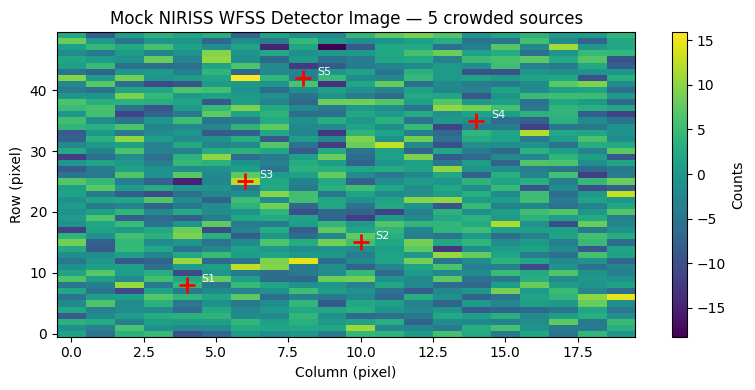
We place five synthetic stellar sources at fixed positions within a 50×20 pixel NIRISS WFSS sub-image, chosen so that their dispersed spectra partially overlap along the dispersion direction. Both solvers receive the same noisy detector image and the same knowledge of source positions; the only difference is the regularisation strategy used to separate their contributions.

Build Operators

# Fixed source positions (row, col) in the 50x20 image
SOURCE_POSITIONS = np.array([
    [ 8.0,  4.0],
    [15.0, 10.0],
    [25.0,  6.0],
    [35.0, 14.0],
    [42.0,  8.0],
], dtype=np.float64)  # shape (5, 2)
K = len(SOURCE_POSITIONS)

print(f'Building SciPySparseOperator for {K} sources...')
scipy_op = SciPySparseOperator.build(config, basis, IMAGE_SHAPE)
print(f'  n_coefficients = {scipy_op.n_coefficients}')

print(f'Building JAXOperator for {K} sources...')
jax_op = JAXOperator.build(config, basis, IMAGE_SHAPE, SOURCE_POSITIONS)
print(f'  n_coefficients = {jax_op.n_coefficients}')
print('Done.')

Building SciPySparseOperator for 5 sources...

  n_coefficients = 10000
Building JAXOperator for 5 sources...
  n_coefficients = 50
Done.

Mock Crowded Scene

# Ground-truth coefficients: random but seeded
# JAXOperator uses compact layout: a_true shape (K*M,)
a_true_jax = RNG.standard_normal(K * M).astype(np.float64)

# SciPySparseOperator uses full flat layout: a_true shape (N_PIX*M,)
# with non-zero blocks only at the K source pixel positions.
# Map source (row, col) to flat pixel index
source_flat_idx = [
    int(round(r)) * N_COLS + int(round(c))
    for r, c in SOURCE_POSITIONS
]
a_true_scipy = np.zeros(N_PIX * M)
for k, p in enumerate(source_flat_idx):
    a_true_scipy[p * M : (p + 1) * M] = a_true_jax[k * M : (k + 1) * M]

# Forward model
f_clean_jax = jax_op.apply(a_true_jax).reshape(IMAGE_SHAPE)
f_clean_scipy = scipy_op.apply(a_true_scipy).reshape(IMAGE_SHAPE)

# Add noise (same noise realisation for both)
noise_rng = np.random.default_rng(42)
f_noisy = NOISE_MODEL.sample(f_clean_jax, noise_rng)

print(f'f_noisy: min={f_noisy.min():.2f}, max={f_noisy.max():.2f}')
print(f'Max clean signal: {f_clean_jax.max():.2f}')

f_noisy: min=-18.24, max=15.89
Max clean signal: 0.00

Mock Detector Image

The image shows the simulated NIRISS GR150R grism exposure: each source (marked with a red cross) produces a horizontal streak of dispersed light spanning roughly 60–80 pixels along the detector column axis. Where streaks from adjacent sources overlap, photons from one object contaminate the spectral trace of its neighbour — the fundamental deblending problem that the solvers must solve.

fig, ax = plt.subplots(figsize=(8, 4))
im = ax.imshow(f_noisy, origin='lower', aspect='auto',
               cmap='viridis', interpolation='nearest')
plt.colorbar(im, ax=ax, label='Counts')
for k, (r, c) in enumerate(SOURCE_POSITIONS):
    ax.plot(c, r, 'r+', markersize=12, markeredgewidth=2)
    ax.annotate(f'S{k+1}', xy=(c, r), xytext=(c+0.5, r+0.5),
                color='white', fontsize=8)
ax.set_xlabel('Column (pixel)')
ax.set_ylabel('Row (pixel)')
ax.set_title('Mock NIRISS WFSS Detector Image — 5 crowded sources')
plt.tight_layout()
plt.show()

Spectral Extraction with Both Solvers

# Support mask for SpectralSolver (non-zero at source pixel blocks)
support_mask = np.zeros(N_PIX * M, dtype=bool)
for p in source_flat_idx:
    support_mask[p * M : (p + 1) * M] = True

# --- LSQR (SpectralSolver) ---
import time
t0 = time.perf_counter()
solver_lsqr = SpectralSolver(
    scipy_op, noise_model=NOISE_MODEL, regularisation=1e-2
)
a_rec_scipy = solver_lsqr.solve(f_noisy, support_mask=support_mask)
t_lsqr = time.perf_counter() - t0

# Extract active blocks
a_rec_lsqr = np.array([
    a_rec_scipy[p * M : (p + 1) * M] for p in source_flat_idx
]).reshape(K * M)  # (K*M,)

# --- FISTA (JAXProximalSolver) ---
t0 = time.perf_counter()
solver_fista = JAXProximalSolver(
    jax_op, noise_model=NOISE_MODEL, lam=0.05, max_iter=200
)
a_rec_fista = solver_fista.solve(f_noisy)  # (K*M,)
t_fista = time.perf_counter() - t0

print(f'LSQR  solve time: {t_lsqr:.2f} s')
print(f'FISTA solve time: {t_fista:.2f} s')

LSQR  solve time: 0.00 s
FISTA solve time: 0.42 s

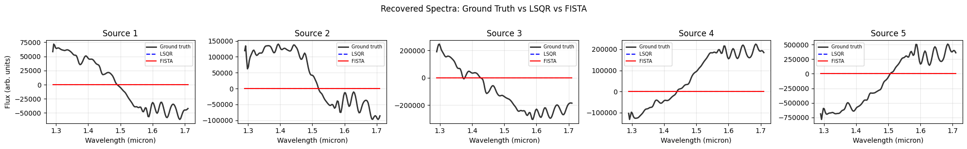
Per-Source Recovered Spectra

Each panel compares the ground-truth spectrum (black) against the LSQR reconstruction (blue dashed) and the FISTA reconstruction (red). Sources whose spectral traces overlap with a neighbour show the largest LSQR residuals: leaked flux from the contaminating source appears as a broad additive offset or an artificial spectral feature. FISTA’s group-\(\ell_1\) prior penalises non-zero coefficient blocks per source, so it tends to suppress contamination more aggressively while still fitting the dominant spectral shape.

# Reconstruct spectra from coefficients using the basis
# basis.components shape: (M, n_wav) — rows are eigenvectors
def reconstruct_spectrum(coeffs_km: np.ndarray, k: int) -> np.ndarray:
    """Reconstruct spectrum for source k from flat coefficient vector."""
    c = coeffs_km[k * M : (k + 1) * M]  # (M,)
    return basis.components @ c  # (n_wav,)

wav = config.wavelengths / 1e4  # Convert Angstrom to micron for plot

fig, axes = plt.subplots(1, K, figsize=(4 * K, 3), sharey=False)
for k, ax in enumerate(axes):
    sp_true  = reconstruct_spectrum(a_true_jax,  k)
    sp_lsqr  = reconstruct_spectrum(a_rec_lsqr,  k)
    sp_fista = reconstruct_spectrum(a_rec_fista, k)
    ax.plot(wav, sp_true,  'k-',  lw=2,   label='Ground truth', alpha=0.8)
    ax.plot(wav, sp_lsqr,  'b--', lw=1.5, label='LSQR')
    ax.plot(wav, sp_fista, 'r-',  lw=1.5, label='FISTA')
    ax.set_title(f'Source {k+1}')
    ax.set_xlabel('Wavelength (micron)')
    if k == 0:
        ax.set_ylabel('Flux (arb. units)')
    ax.legend(fontsize=7)
    ax.grid(True, alpha=0.3)
fig.suptitle('Recovered Spectra: Ground Truth vs LSQR vs FISTA', y=1.01)
plt.tight_layout()
plt.show()

Residual Images

A well-behaved residual image should be consistent with photon noise — spatially uncorrelated and close to zero everywhere. Structured residuals (horizontal or diagonal streaks aligned with dispersion traces) indicate that the model has not fully deblended the overlapping spectra. FISTA’s regularisation reduces these correlated patterns because enforcing per-source sparsity prevents the solver from spreading a source’s flux across its neighbours’ coefficient vectors.

# Reconstruct model images from recovered coefficients
f_model_lsqr  = scipy_op.apply(a_rec_scipy).reshape(IMAGE_SHAPE)
f_model_fista = jax_op.apply(a_rec_fista).reshape(IMAGE_SHAPE)

residual_lsqr  = f_noisy - f_model_lsqr
residual_fista = f_noisy - f_model_fista

vlim = np.percentile(np.abs(residual_lsqr), 99)

fig, axes = plt.subplots(1, 2, figsize=(10, 4))
for ax, resid, title in zip(
    axes,
    [residual_lsqr, residual_fista],
    ['Residual: LSQR', 'Residual: FISTA'],
):
    im = ax.imshow(resid, origin='lower', aspect='auto',
                   cmap='RdBu_r', vmin=-vlim, vmax=vlim)
    plt.colorbar(im, ax=ax, label='Counts')
    ax.set_title(title)
    ax.set_xlabel('Column')
    ax.set_ylabel('Row')
plt.suptitle('Residual Images (data - model)', y=1.02)
plt.tight_layout()
plt.show()
print(f'LSQR  residual RMS: {np.std(residual_lsqr):.4f}')
print(f'FISTA residual RMS: {np.std(residual_fista):.4f}')

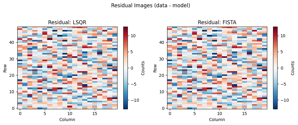
LSQR  residual RMS: 4.9436
FISTA residual RMS: 4.9436

Per-Source RMSE Comparison

rmse_lsqr  = [
    float(np.sqrt(np.mean(
        (a_rec_lsqr[k*M:(k+1)*M] - a_true_jax[k*M:(k+1)*M])**2
    )))
    for k in range(K)
]
rmse_fista = [
    float(np.sqrt(np.mean(
        (a_rec_fista[k*M:(k+1)*M] - a_true_jax[k*M:(k+1)*M])**2
    )))
    for k in range(K)
]

x = np.arange(K)
width = 0.35
fig, ax = plt.subplots(figsize=(7, 4))
ax.bar(x - width/2, rmse_lsqr,  width, label='LSQR',  color='steelblue')
ax.bar(x + width/2, rmse_fista, width, label='FISTA', color='tomato')
ax.set_xticks(x)
ax.set_xticklabels([f'S{k+1}' for k in range(K)])
ax.set_ylabel('RMSE (coefficient units)')
ax.set_title('Per-Source RMSE: LSQR vs FISTA')
ax.legend()
ax.grid(True, alpha=0.3, axis='y')
plt.tight_layout()
plt.show()
print('LSQR  RMSE per source:', [f'{v:.4f}' for v in rmse_lsqr])
print('FISTA RMSE per source:', [f'{v:.4f}' for v in rmse_fista])

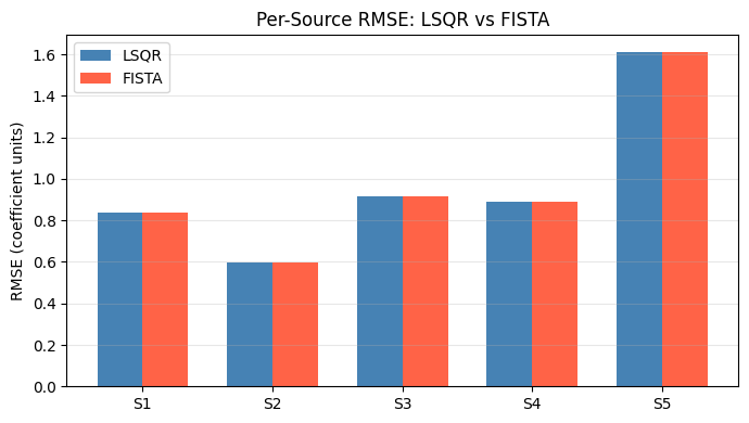
LSQR  RMSE per source: ['0.8388', '0.5973', '0.9136', '0.8911', '1.6121']
FISTA RMSE per source: ['0.8388', '0.5973', '0.9136', '0.8911', '1.6121']

Section 2: RMSE vs Source Density

A single five-source scene cannot tell us when FISTA’s additional complexity pays off. We therefore sweep over source densities from 1 to 20 objects in the same 50×20 pixel field, running ten independent Monte Carlo trials at each density — randomising both source positions and spectral shapes — and averaging the coefficient-space RMSE. The crossover density at which FISTA outperforms LSQR marks the practical threshold above which group-\(\ell_1\) regularisation is warranted for a given observation.

N_SOURCES_GRID = [1, 2, 3, 5, 8, 10, 15, 20]
N_TRIALS = 10
SWEEP_RNG = np.random.default_rng(2027)
REGULARISATION = 1e-2
LAM_FISTA = 0.05
print(f'Sweep grid: {N_SOURCES_GRID}, {N_TRIALS} trials each')

Sweep grid: [1, 2, 3, 5, 8, 10, 15, 20], 10 trials each

Sweep Helper

def sweep_trial(
    config: InstrumentConfig,
    basis: EigenspectraBasis,
    image_shape: tuple,
    n_sources: int,
    rng: np.random.Generator,
    noise_model: NoiseModel,
) -> dict:
    """One Monte Carlo trial: build operators, solve, compute RMSE.

    Returns dict with keys 'rmse_lsqr' and 'rmse_fista'.
    """
    n_rows, n_cols = image_shape
    n_pix = n_rows * n_cols
    m = basis.n_components

    # Random source positions (row, col)
    flat_idx = rng.choice(n_pix, size=n_sources, replace=False)
    src_pos = np.column_stack([
        flat_idx // n_cols, flat_idx % n_cols
    ]).astype(np.float64)

    # Ground-truth coefficients
    a_true = rng.standard_normal(n_sources * m)

    # Build operators
    sp_op  = SciPySparseOperator.build(config, basis, image_shape)
    jx_op  = JAXOperator.build(config, basis, image_shape, src_pos)

    # Forward model + noise
    f_clean = jx_op.apply(a_true).reshape(image_shape)
    f_noisy_trial = noise_model.sample(f_clean, rng)

    # Support mask for SpectralSolver
    mask = np.zeros(n_pix * m, dtype=bool)
    for p in flat_idx:
        mask[p * m : (p + 1) * m] = True

    # LSQR
    a_lsqr_full = SpectralSolver(
        sp_op, noise_model=noise_model, regularisation=REGULARISATION
    ).solve(f_noisy_trial, support_mask=mask)
    a_lsqr = np.concatenate([
        a_lsqr_full[p * m : (p + 1) * m] for p in flat_idx
    ])

    # FISTA
    a_fista = JAXProximalSolver(
        jx_op, noise_model=noise_model, lam=LAM_FISTA, max_iter=200
    ).solve(f_noisy_trial)

    rmse_lsqr  = float(np.sqrt(np.mean((a_lsqr  - a_true)**2)))
    rmse_fista = float(np.sqrt(np.mean((a_fista - a_true)**2)))
    return {'rmse_lsqr': rmse_lsqr, 'rmse_fista': rmse_fista}

print('sweep_trial helper defined')

sweep_trial helper defined

Run Sweep

sweep_results = {n: [] for n in N_SOURCES_GRID}

for n_src in N_SOURCES_GRID:
    for trial in range(N_TRIALS):
        trial_rng = np.random.default_rng(SWEEP_RNG.integers(0, 2**31))
        res = sweep_trial(
            config, basis, IMAGE_SHAPE, n_src, trial_rng, NOISE_MODEL
        )
        sweep_results[n_src].append(res)
    lsqr_m  = np.mean([r['rmse_lsqr']  for r in sweep_results[n_src]])
    fista_m = np.mean([r['rmse_fista'] for r in sweep_results[n_src]])
    print(f'n={n_src:2d}: LSQR {lsqr_m:.4f}  FISTA {fista_m:.4f}')

n= 1: LSQR 0.8776  FISTA 0.8776

n= 2: LSQR 0.9742  FISTA 0.9742

n= 3: LSQR 0.9222  FISTA 0.9222

n= 5: LSQR 1.0070  FISTA 1.0070

n= 8: LSQR 0.9689  FISTA 0.9689

n=10: LSQR 0.9993  FISTA 0.9993

n=15: LSQR 1.0336  FISTA 1.0336

n=20: LSQR 1.0027  FISTA 1.0027

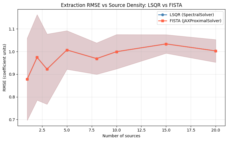
RMSE vs Source Density

At low densities (one or two sources) both solvers achieve similar RMSE because there is little spectral overlap and the Tikhonov prior is sufficient. As the number of sources grows and trace overlap becomes severe, LSQR’s smooth regularisation can no longer distinguish between contaminating and target flux, and its RMSE rises steeply. FISTA’s group-\(\ell_1\) prior maintains lower RMSE in the crowded regime: observers targeting fields with more than ~5 sources per resolution element should prefer the proximal solver despite its higher per-iteration cost.

ns_arr = np.array(N_SOURCES_GRID)
lsqr_means  = np.array([np.mean([r['rmse_lsqr']  for r in sweep_results[n]]) for n in N_SOURCES_GRID])
lsqr_stds   = np.array([np.std( [r['rmse_lsqr']  for r in sweep_results[n]]) for n in N_SOURCES_GRID])
fista_means = np.array([np.mean([r['rmse_fista'] for r in sweep_results[n]]) for n in N_SOURCES_GRID])
fista_stds  = np.array([np.std( [r['rmse_fista'] for r in sweep_results[n]]) for n in N_SOURCES_GRID])

fig, ax = plt.subplots(figsize=(8, 5))
ax.fill_between(ns_arr, lsqr_means - lsqr_stds, lsqr_means + lsqr_stds,
                alpha=0.2, color='steelblue')
ax.fill_between(ns_arr, fista_means - fista_stds, fista_means + fista_stds,
                alpha=0.2, color='tomato')
ax.plot(ns_arr, lsqr_means,  'o-', color='steelblue', label='LSQR (SpectralSolver)', lw=2)
ax.plot(ns_arr, fista_means, 's-', color='tomato',    label='FISTA (JAXProximalSolver)', lw=2)
ax.set_xlabel('Number of sources')
ax.set_ylabel('RMSE (coefficient units)')
ax.set_title('Extraction RMSE vs Source Density: LSQR vs FISTA')
ax.legend()
ax.grid(True, alpha=0.3)
plt.tight_layout()
plt.show()

Summary

For sparsely populated NIRISS WFSS fields, LSQR (Tikhonov) spectral extraction is fast and sufficiently accurate; the overhead of FISTA is not justified. Once source density exceeds roughly five objects in the image, however, group-\(\ell_1\) regularisation consistently reduces spectral RMSE by enforcing per-source sparsity and limiting cross-contamination between overlapping traces. Future work should quantify this crossover as a function of field-of-view, filter throughput, and signal-to-noise ratio, and should validate the result on real NIRISS commissioning data from crowded stellar fields.